| (Caffe,LeNet)反向传播(六) | 您所在的位置:网站首页 › 反向传播算法 推导图片 › (Caffe,LeNet)反向传播(六) |
(Caffe,LeNet)反向传播(六)
|
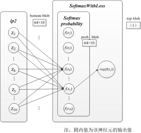
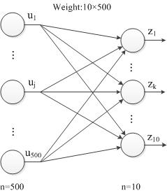
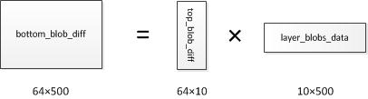
本文地址:http://blog.csdn.net/mounty_fsc/article/details/51379395 本部分剖析Caffe中Net::Backward()函数,即反向传播计算过程。从LeNet网络角度出发,且调试网络为训练网络,共9层网络。具体网络层信息见 (Caffe,LeNet)初始化训练网络(三) 第2部分 本部分不介绍反向传播算法的理论原理,以下介绍基于对反向传播算法有一定的了解。 1 入口信息Net::Backward()函数中调用BackwardFromTo函数,从网络最后一层到网络第一层反向调用每个网络层的Backward。 void Net::BackwardFromTo(int start, int end) { for (int i = start; i >= end; --i) { if (layer_need_backward_[i]) { layers_[i]->Backward( top_vecs_[i], bottom_need_backward_[i], bottom_vecs_[i]); if (debug_info_) { BackwardDebugInfo(i); } } } } 2 第九层SoftmaxWithLossLayer 2.1 代码分析代码实现如下: void SoftmaxWithLossLayer::Backward_gpu(const vector& top, const vector& propagate_down, const vector& bottom) { // bottom_diff shape:64*10 Dtype* bottom_diff = bottom[0]->mutable_gpu_diff(); // prob_data shape:64*10 const Dtype* prob_data = prob_.gpu_data(); // top_data shape:(1) const Dtype* top_data = top[0]->gpu_data(); // 将Softmax层预测的结果prob复制到bottom_diff中 caffe_gpu_memcpy(prob_.count() * sizeof(Dtype), prob_data, bottom_diff); // label shape:64*1 const Dtype* label = bottom[1]->gpu_data(); // dim = 640 / 64 = 10 const int dim = prob_.count() / outer_num_; // nthreads = 64 / 1 = 64 const int nthreads = outer_num_ * inner_num_; // Since this memory is never used for anything else, // we use to to avoid allocating new GPU memory. Dtype* counts = prob_.mutable_gpu_diff(); // 该函数将bottom_diff(此时为每个类的预测概率)对应的正确类别(label)的概率值-1,其他数据没变。见公式推导。 SoftmaxLossBackwardGPU(nthreads, top_data, label, bottom_diff, outer_num_, dim, inner_num_, has_ignore_label_, ignore_label_, counts); // 代码展开开始,代码有修改 __global__ void SoftmaxLossBackwardGPU(...) { CUDA_KERNEL_LOOP(index, nthreads) { const int label_value = static_cast(label[index]); bottom_diff[index * dim + label_value] -= 1; counts[index] = 1; } } // 代码展开结束 Dtype valid_count = -1; // 注意为loss的权值,对该权值(一般为1或者0)归一化(除以64) // Scale gradient const Dtype loss_weight = top[0]->cpu_diff()[0]; if (normalize_) { caffe_scal(prob_.count(), loss_weight / count, bottom_diff); } else { caffe_scal(prob_.count(), loss_weight / outer_num_, bottom_diff); } }说明: 1. SoftmaxWithLossLayer是没有学习参数的(见前向计算(五)) ,因此不需要对该层的参数做调整,只需要计算bottom_diff(理解反向传播算法的链式求导,求bottom_diff对上一层的输出求导,是为了进一步计算调整上一层权值) 2. 以上代码核心部分在SoftmaxLossBackwardGPU。该函数将bottom_diff(此时为每个类的预测概率)对应的正确类别(label)的概率值-1,其他数据没变。这里使用前几节的符号系统及图片进行解释。 2.2 公式推导符号系统 设SoftmaxWithLoss层的输入为向量 z ,即bottom_blob_data,也就是上一层的输出。经过Softmax计算后的输出为向量 f(z) ,公式为(省略了标准化常量m) f(zk)=ezk∑niezi 。最后SoftmaxWithLoss层的输出为 loss=∑n−logf(zy) , y 为样本的标签。见前向计算(五)。 反向推导 把loss展开可得 loss=log∑inezi−zy 所以 dlossdz 结果如下: ∂loss∂zi={f(zy)−1,zi=zyf(zi),zi≠zy图示 如图,当前层ip2层的输入为 z ,上一层的输入为 u 。 1. 对上一层输出求偏导 ∂loss∂uj 存放在ip2层的bottom_blob_diff(64*500)中,计算公式如下,其中 ∂loss∂zk 存放在top_blob_diff(64*10)中: ∂zk∂uj=∑100jwkjuj∂uj=wkj ∂loss∂uj=∑kn=10∂loss∂zk∂zk∂uj=∑kn=10∂loss∂zkwkj 写成向量的形式为: ∂loss∂uj=∂loss∂zT⋅wj 进一步,写成矩阵的形式,其中 u 为500维, z 为10维, W 为 10×500 : ∂loss∂uT=∂loss∂zT⋅W 再进一步,考虑到一个batch有64个样本,表达式可以写成如下形式,其中 U 为 64×500 ; Z 为 64×10 ; W 为 10×500 : ∂loss∂U=∂loss∂Z⋅W2. 对参数求偏导 ∂loss∂wkj=∂loss∂zk∂zk∂wkj=∂loss∂zkuj 写成向量的形式有: ∂loss∂wj=∂loss∂zuj 进一步,可以写成矩阵形式,其中 W 为 10×500 ; z 为10维; u 为500维。 ∂loss∂W=∂loss∂zuT 再进一步,考虑到一个batch有64个样本,表达式可以写成如下形式,其中 W 为 10×500 ; Z 为 64×10 ; U 为 64×500 : ∂loss∂W=∂loss∂ZT⋅U 4 第七层ReLU
4.1 代码分析
4 第七层ReLU
4.1 代码分析
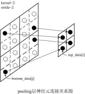
cpu代码分析如下,注,该层没有参数,只需对输入求导 void ReLULayer::Backward_cpu(const vector& top, const vector& propagate_down, const vector& bottom) { if (propagate_down[0]) { const Dtype* bottom_data = bottom[0]->cpu_data(); const Dtype* top_diff = top[0]->cpu_diff(); Dtype* bottom_diff = bottom[0]->mutable_cpu_diff(); const int count = bottom[0]->count(); //见公式推导 Dtype negative_slope = this->layer_param_.relu_param().negative_slope(); for (int i = 0; i < count; ++i) { bottom_diff[i] = top_diff[i] * ((bottom_data[i] > 0) + negative_slope * (bottom_data[i] top_diffitop_diffi∗slopebottom_datai>0bottom_datai≤0 5 第五层Pooling 5.1 代码分析Maxpooling的cpu代码分析如下,注,该层没有参数,只需对输入求导 void PoolingLayer::Backward_cpu(const vector& top, const vector& propagate_down, const vector& bottom) { const Dtype* top_diff = top[0]->cpu_diff(); Dtype* bottom_diff = bottom[0]->mutable_cpu_diff(); // bottom_diff初始化置0 caffe_set(bottom[0]->count(), Dtype(0), bottom_diff); const int* mask = NULL; // suppress warnings about uninitialized variables ... // 在前向计算时max_idx中保存了top_data中的点是有bottom_data中的点得来的在该feature map中的坐标 mask = max_idx_.cpu_data(); // 主循环,按(N,C,H,W)方式便利top_data中每个点 for (int n = 0; n < top[0]->num(); ++n) { for (int c = 0; c < channels_; ++c) { for (int ph = 0; ph < pooled_height_; ++ph) { for (int pw = 0; pw < pooled_width_; ++pw) { const int index = ph * pooled_width_ + pw; const int bottom_index = mask[index]; // 见公式推导 bottom_diff[bottom_index] += top_diff[index]; } } bottom_diff += bottom[0]->offset(0, 1); top_diff += top[0]->offset(0, 1); mask += top[0]->offset(0, 1); } } } 5.2 公式推导由图可知,maxpooling层是非线性变换,但有输入与输出的关系可线性表达为 bottom_dataj=top_datai (所以需要前向计算时需要记录索引i到索引j的映射max_idx_. 链式求导有: bottom_diffj=∂loss∂bottom_dataj=∂loss∂top_datai⋅∂top_datai∂bottom_dataj=top_diffi⋅1(注意下标) 6 第四层Convolution void ConvolutionLayer::Backward_cpu(const vector& top, const vector& propagate_down, const vector& bottom) { const Dtype* weight = this->blobs_[0]->cpu_data(); Dtype* weight_diff = this->blobs_[0]->mutable_cpu_diff(); for (int i = 0; i < top.size(); ++i) { const Dtype* top_diff = top[i]->cpu_diff(); const Dtype* bottom_data = bottom[i]->cpu_data(); Dtype* bottom_diff = bottom[i]->mutable_cpu_diff(); // Bias gradient, if necessary. if (this->bias_term_ && this->param_propagate_down_[1]) { Dtype* bias_diff = this->blobs_[1]->mutable_cpu_diff(); // 对于每个Batch中的样本,计算偏置的偏导 for (int n = 0; n < this->num_; ++n) { this->backward_cpu_bias(bias_diff, top_diff + n * this->top_dim_); } } if (this->param_propagate_down_[0] || propagate_down[i]) { // 对于每个Batch中的样本,关于权值及输入求导部分代码展开了函数(非可运行代码) for (int n = 0; n < this->num_; ++n) { // gradient w.r.t. weight. Note that we will accumulate diffs. //top_diff(50*64) * bottom_data(500*64,Transpose) = weight_diff(50*500) // 注意,此处(Dtype)1., this->blobs_[0]->mutable_gpu_diff() // 中的(Dtype)1.:使得在一个solver的iteration中的多个iter_size // 的梯度没有清零,而得以累加 caffe_cpu_gemm(CblasNoTrans, CblasTrans, conv_out_channels_ / group_, kernel_dim_, conv_out_spatial_dim_, (Dtype)1., top_diff + n * this->top_dim_, bottom_data + n * this->bottom_dim_, (Dtype)1., weight_diff); // gradient w.r.t. bottom data, if necessary. // weight(50*500,Transpose) * top_diff(50*64) = bottom_diff(500*64) caffe_cpu_gemm(CblasTrans, CblasNoTrans, kernel_dim_, conv_out_spatial_dim_, conv_out_channels_ , (Dtype)1., weight, top_diff + n * this->top_dim_, (Dtype)0., bottom_diff + n * this->bottom_dim_); } } } }说明: 第四层的bottom维度 (N,C,H,W)=(64,20,12,12) ,top的维度bottom维度 (N,C,H,W)=(64,50,8,8) ,由于每个样本单独处理,所以只需要关注 (C,H,W) 的维度,分别为 (20,12,12) 和 (50,8,8) 根据(Caffe)卷积的实现,该层可以写成矩阵相乘的形式 Weight_data×Bottom_dataT=Top_data Weight_data 的维度为 Cout×(C∗K∗K)=50×500 Bottom_data 的维度为 (H∗W)×(C∗K∗K)=64×500 , 64 为 8∗8 个卷积核的位置, 500=C∗K∗K=20∗5∗5 Top_data 的维度为 64×50 写成矩阵表示后,从某种角度上与全连接从(也是表示成矩阵相乘)相同,因此,可以借鉴全连接层的推导。 |
【本文地址】